The VLOOKUP function is one of the staple functions that Microsoft Excel users rely upon for finding values in a table. With the VLOOKUP function, a value can be looked up in the leftmost column and a related value can be returned from another column.

The Syntax for VLOOKUP is VLOOKUP(lookup_value, table_array, col_index_num, [range_lookup])

• Lookup Value: the criteria, which may be an id or key, that is being searched for in the farthest left column
• Table Array: range containing of the table that is being looked through. It must include the criteria column as well as the output column desired.
• Col index number: the column number of the output column, where column 1 is the leftmost column of the Table Array containing the Lookup Value.
• Range lookup: a Boolean parameter that allows for approximate matches. The default value is TRUE, which allows for approximate matches. FALSE requires an exact match. When set to TRUE, only the first approximate match is found so the table must be sorted for it to operate as expected. Why and when you would want to do approximate matches will be covered later.

VLOOKUP with EXACT MATCH

The VLOOKUP function is most often used to find a value that is related to an exact value.

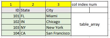
To lookup the City in this table for ID 103, the formula is
=VLOOKUP(103,B6:D9,3,0)
To find the State, change col index num from 3 to 2.
The City can also be found by looking up the State. In this case, the table array definition must be changed so that the State is in the left most column, as follows:
=VLOOKUP(“FL”,C6:D9,2,0)
For an exact match, the value in the first column is assumed to be unique. If it is not, VLOOKUP will only return the first match, which is one of its shortcomings. The data in the left most column of the array must be evaluated or tested for uniqueness when using a VLOOKUP with an exact match.

VLOOKUP APPROXIMATE MATCHING
At first, finding an approximate match sounds like a great idea but Excel doesn’t indicate why or how close of a match it finds. Unlike SQL, which you may be familiar with, Excel doesn’t have a formula that calculates and sorts based on the closeness of the match. Instead, Excel’s VLOOKUP returns the first approximate match it finds when searching down a column from top to bottom. So how can this be useful?

If you were to go to the support page for Microsoft Office and look at the entire write up for VLOOKUP, you would find advice and examples concerning approximate matching with VLOOKUP to be lacking. As of this writing, of the 6 examples listed and the 2 minute video about VLOOKUP, not one approximate matching example is provided even though it is one of the most powerful features.

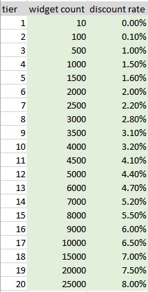
Let’s pose a scenario. Your company offers tiered pricing of widgets, based on the quantity purchased. There are 20 tiers of different widget counts and discount rates. If you were so inclined, you could handle this with a hefty IF formula, such as this:

=IF(A1>25000,8%,IF(A1>20000,7.5%,IF(A1>15000,7.0%,IF(A1>10000,6.5%, IF(A1>9000,6.0%,IF(A1>8000,5.5%,IF(A1>7000,5.2%,IF(A1>6000,4.7%, IF(A1>6000,4.7%,IF(A1>5000,4.4%,IF(A1>4500,4.1%,IF(A1>4000,3.2%, IF(A1>3500,3.1%,IF(A1>3000,2.8%,IF(A1>2500,2.2%,IF(A1>2000,2%, IF(A1>1500,1.6%,IF(A1>1000,1.5%,IF(A1>500,1%,IF(A1>100,.1%,0%))))))))))))))))))))

The above formula will not work exactly as written, but is just provided to illustrate the complexity of the formula needed for this purpose.

A better alternative is to use a sorted table and an approximate VLOOKUP match. First, set up the table with the 20 tiers and sort the table smallest to largest, as in the example below.

If necessary, this pricing table can be placed in a hidden worksheet and protected from unauthorized changes. The table can also be populated through a data connection to a SharePoint list. A SharePoint list has several advantages, including the following:

• Only users with permissions can connect to sensitive pricing information stored in SharePoint
• When pricing information is updated in SharePoint, all Excel workbooks connected to that list are automatically updated the next time they are opened and the connections are refreshed.

The best practice is to give the table a reference name (see the Defined names section of the Formulas Tab in the ribbon.) In the following examples, the green highlighted range of B5:C24 has been given the name WIDGET_RATES. Note that the VLOOKUP will use a lookup value of widget count, so widget count must be in the leftmost column of the WIDGET_RATES array.
This time, instead of a massive nest IF formula, a much shorter formula can be used to find the appropriate discount rate:

VLOOKUP(widgetcount,WIDGET_RATES,2)

Since the default operation of VLOOKUP is the approximate match, the final parameter can be omitted.

This approximate VLOOKUP will scan down the list looking for the first approximate match in widget count and will return the discount rate.

For the formula below, 1000 is the closest match and the formula returns 1.5%.

VLOOKUP(1100,WIDGET_RATES,2)

For the formula below, although 2500 appears to be the closest match to 2499, the VLOOKUP formula will return the value of 2% for anything in the range of 2000 up to, but not including, 2500.

VLOOKUP(2499,WIDGET_RATES,2)

The great strength in substituting an approximate VLOOKUP for a complex, nested IF statement is that changes can be made to the table without ever needing to alter the VLOOKUP formula. Using a nested If statement, should a new tier need to be added or tiers removed, the formula would need to be expanded or contracted, a tedious process even for the seasoned Excel user.
This approximate match method also works with text strings. Consider the following table.

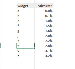
VLOOKUP(“d”,WIDGET_RATES,2) would return 0.1% as d is > c but it is not equal to an e.

The difference between capital and lowercase does not matter to VLOOKUP, it treats all text as a single case.

UNIQUE LOOKUP TRICK WITH VLOOKUP

With the VLOOKUP formula, values in the leftmost column of the table_array must be unique. If these values are not unique, an incorrect match can occur. One way to avoid this scenario is by creating a key column.

A key column can be created by concatenating values in other columns to create a unique identifier. This works especially well when dealing with lists of people. Although multiple people can have the same name, concatenating the first name, last name, city name and job title greatly reduces the chance of duplicates. Consider the example below with three individuals named John Smith and yellow highlighted ID column that has been added, using the formula =C5&D5&E5, to provide a unique ID field:

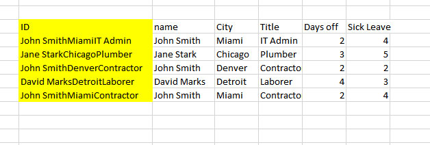
Using a VLOOKUP that searched the name column for John Smith, would have returned a value related to first John Smith encountered in the name column, the IT Admin in Miami. Using the unique ID field, we can search for John SmithMiamiContractor and the value relating to that person will be returned.