Building a Pivot Table in Microsoft Excel: Article 2

In this article, the second in our series on PivotTables, we will show you how to build the simple PivotTable pictured in the introduction.

The first step is to insert the table and pick the data that will be used to populate the table.You can select a PivotTable from the Insert ribbon, as pictured.

Once you select the PivotTable option, Excel will show the following window:

First, select a Table/Range.You can enter the cell range, hit the range select button and highlight the table, or type in the name of your range.

Then, choose the location by inserting the pivot into a new worksheet or the current seleted cell (“Existing Worksheet”).

Press OK, and you are ready to construct your first pivot table!If you remember from the introduction, our data is from a hypothetical entrepreneur who operates his own tax preparation business. After completing the previous steps, we must choose the Fields.

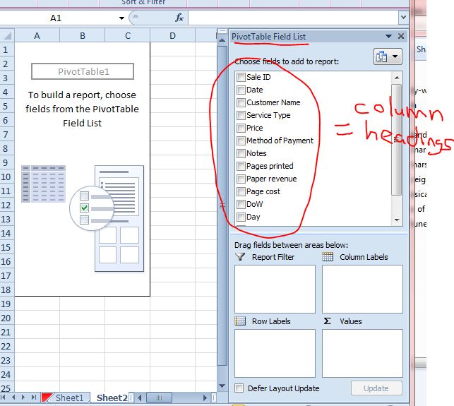
What is a field? In the table containing your data, fields are equivalent to columns. The options in the PivotTable Field List are the headings for the table columns. Not only is it good practice in general, but for constructing pivot table it is a must that you organize your spreadsheets with the fields as columns and each row representing a record. Furthermore, do not leave any blank rows or columns within your table.

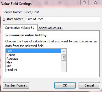
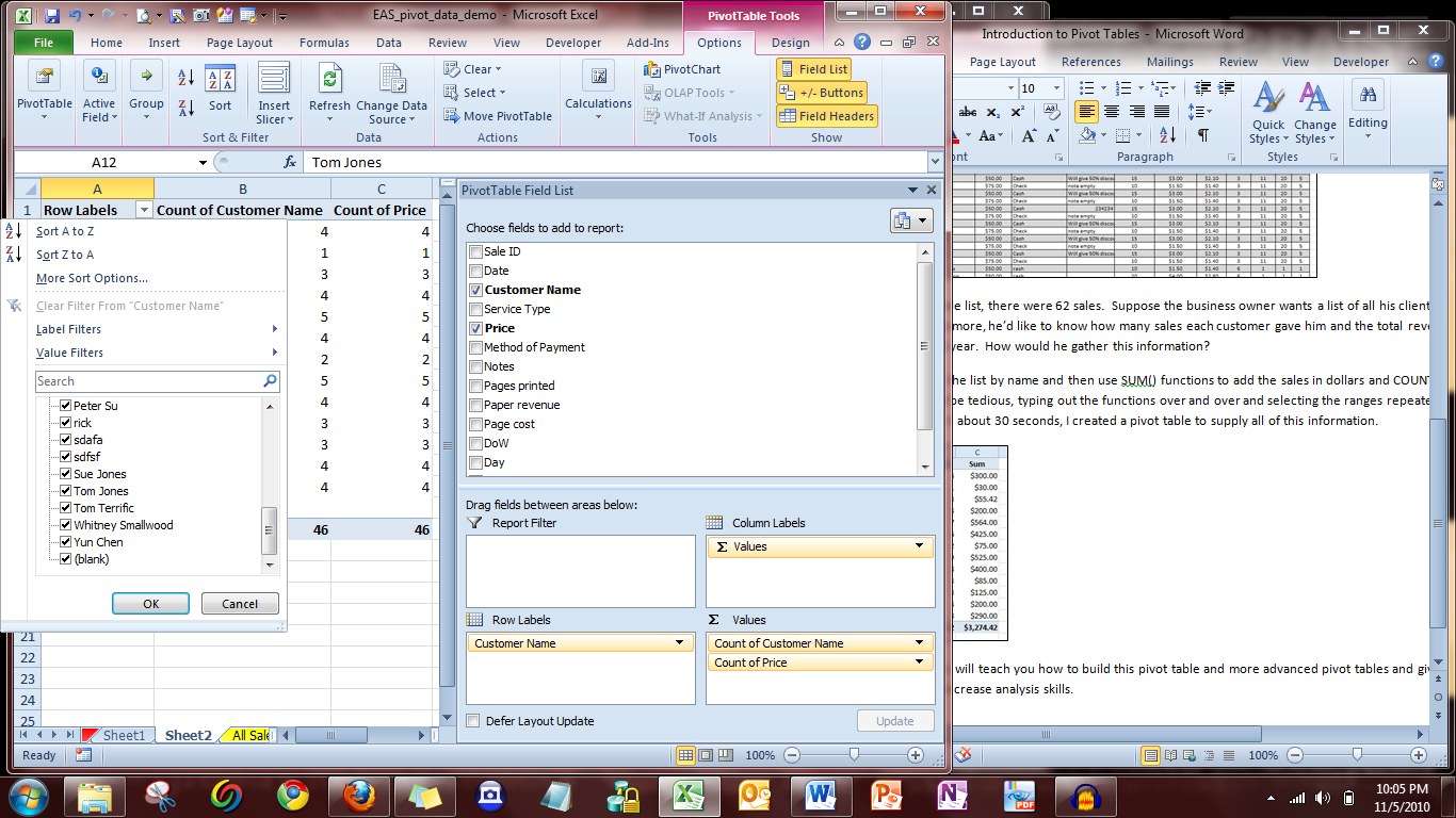
Our entrepreneur, in order to build his customer list, needs information on the names of Customers, how many times each name occurs, and the price each is charged per sale.All of this information is contained within the fields and we must choose to place them in the following areas: Report Filter, Column Labels, Row Labels, and Values.The basic customer list includes Customer Name in the Row labels, Customer Name in the Values, and Price in the Values area.He also removed a “blank” row at the bottom by selecting the Row Label drop down button and unchecking “blank” (all of this is shown in a picture at the end of the article).Finally, Price must not be a count but a sum.This can be changed via the drop down next to a field name under Value Field Settings.Whereas Count would only report the number of entries in the Price Column (which would be equal to the number of transactions per person, information we already obtain by Counting the names), Sum will add the total sales for every transaction of each customer.

The last step to create this basic PivotTable is to format the data itself.You can change the field names (i.e. Column Headings) by editing the text as you would in any other cell.This can be useful as the purpose of a pivot table may be furthered by giving the fields more specific names than that of your source table column headings.We also added the Currency format to the Price field in order that the entrepreneur could see his customer revenues expressed in dollars.

Now that you know what a PivotTable is, why to use it, and how to create a basic PivotTable, we will explore many of the PivotTable options available and then construct more advanced Tables.