
Tables come in many styles and formats. For reporting purposes, the better a table is formatted, the easier it is to read. However, formatting is often our enemy when we attempt to use the data for analysis, database, and data integration purposes. In this blog post, we will demonstrate how to unformat a table and turn it into a backend data table that is ready for other uses.
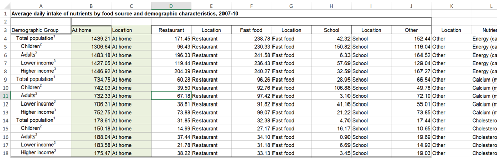
Below is a perfect example of a well-formatted table. It has a title, clearly labeled row and column headings/subheadings, numbers with 2 decimal places, and footnotes. This table is a truncated version of a larger table from the source cited. For the purpose of data preparation, our goal is to convert this into a table with single column headings and data, but no row headings or subheadings.
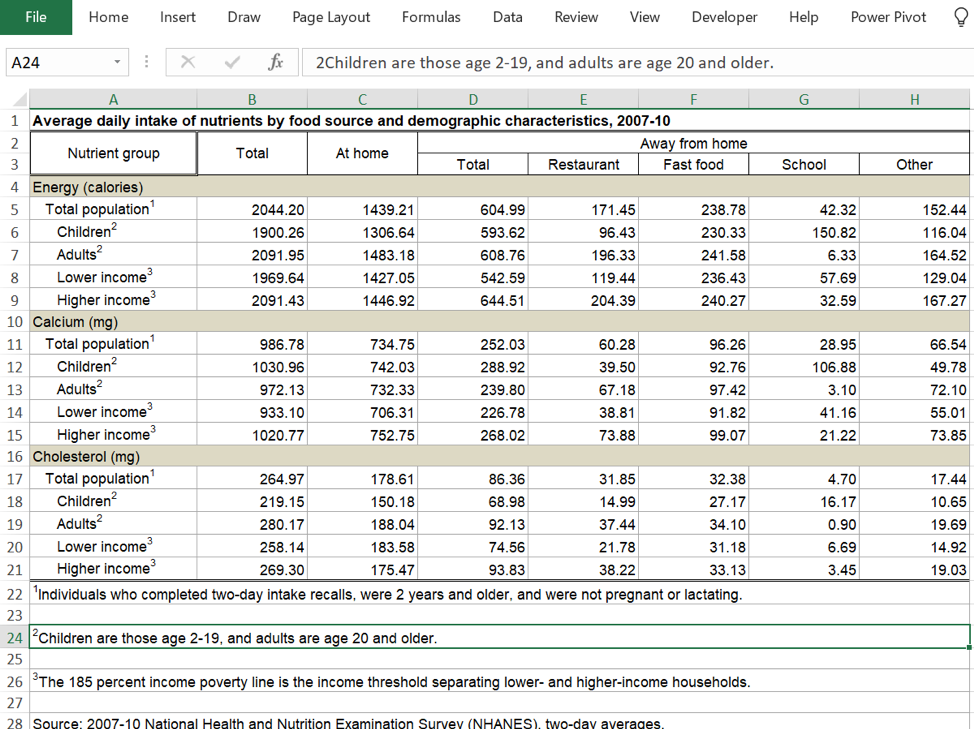
Source: https://www.ers.usda.gov/webdocs/DataFiles/50590/nutrient_table1.xls?v=0
Step 1: Unmerge Cells in Row and Column Headings
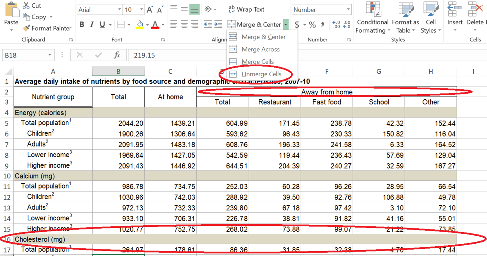
The first step is to unmerge all merged cells in the table. For this table, there are merged cells in the column header, and in each taupe colored bar designating the nutrient groups.
Step 2: Rearrange Table
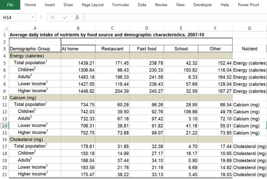
In the above image, columns B and D contain totals that are calculated from values in other columns. These columns can be deleted because the totals can always be obtained again by recalculating. Also, add a new field called Nutrient, in column G, in preparation for eliminating the Nutrient subheadings. Populate the Nutrient field with the appropriate text. Add “Demographic Group” as a heading for Column A. The rearranged table should now look like this:
Step 3: Delete Rows with the Nutrient Subheadings
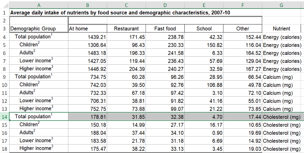
After deleting the taupe shaded rows with the Nutrient subheadings, the table should look like this:
Step 4: Prepare Columns for Transformation to 2 Columns
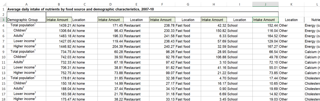
In the above table, the 5 headers of “At Home” to “Other” (Columns B through F) are all related to the location where the nutrients were consumed. As a result, the header descriptions will become values of a location field. The 5 columns will become 2 columns: Location and Intake Amount. To prepare the table for this transformation, we will add Location columns and populate them with the location from the adjacent header, as shown in the green highlighted cells below.
The second part of this step is to rename the “At home,” “Restaurant,” “Fast Food,” “School,” and “Other” headers to “Intake Amount.” This will reflect that those columns contain the intake values associated with the location that is now in the Location column.
Step 5: Transform the Table
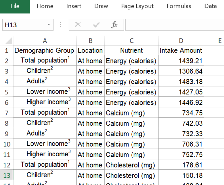
At this point, we’re close to having a final data table with 4 columns: Demographic Group, Location, Nutrient, and Intake Amount. All we need to do is transform it a bit more and rearrange the columns. Once done, it looks like the image below. Our truncated table that contained 20 rows of data in 8 columns now contains 75 rows of data in 4 columns.
Step 6: Dress it Up
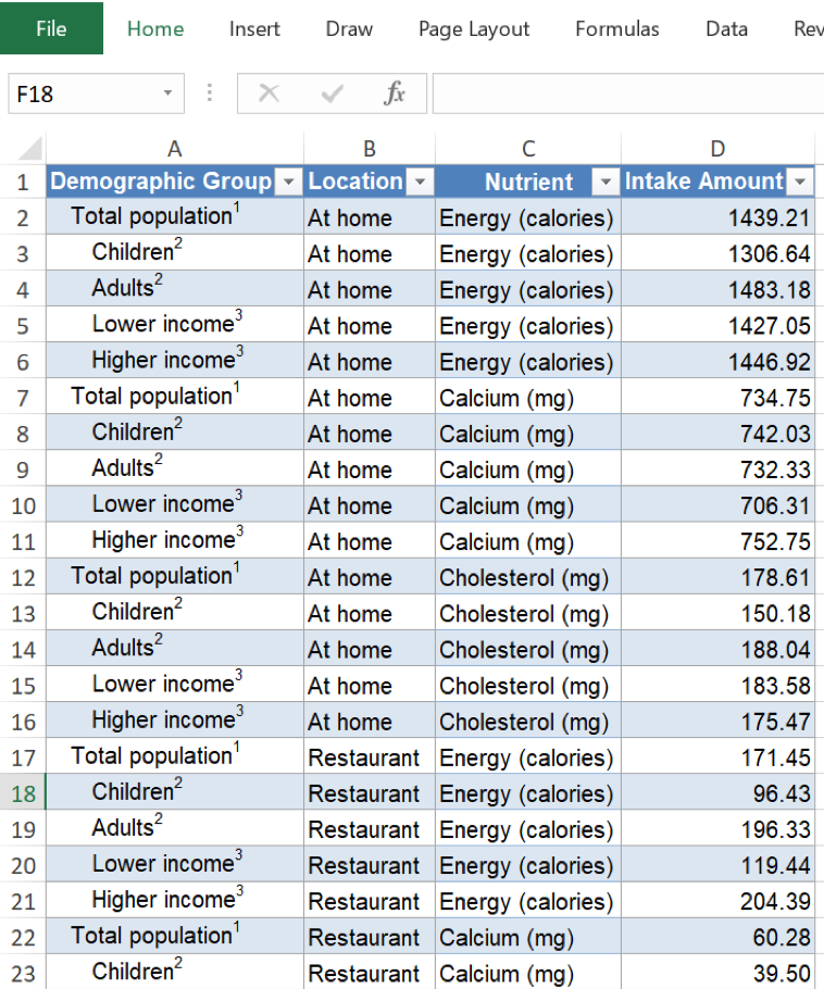
Now that the data is extracted and in usable format, you can convert it into a table. While in any cell within the table, press Ctrl A to select the whole table. Then select the Insert Tab and select “Table.” Check the box next to “My Table has Headers.” Now your table can easily be sorted or appended:
Step 7: Process Automation
If the above steps seem tedious and time consuming, there is a better way, especially if you need to transform the same type of data repeatedly. With VBA programming and the experts at ExcelHelp.com, your data transformation tasks can be automated and completed with the click of a button.
Contact ExcelHelp.com for A Free Consultation
Let us help you design and develop a rock-solid solution for your firm. Contact our team to schedule a free consultation by calling 1-800-682-0882 or visit our website at ExcelHelp.com to submit an inquiry online.